13 Oct 2018

Naive Bayes Classifier

A probabilistic classifier using Gaussian class-conditionals

Fig. 1 - There are three data sets labeled A, B, and C. The goal is to understand the class distributions such that when new unlabeled data are presented (red circles labeled 1-3), a class may be assigned based on probability. In this example, the new data point labeled as 1 has an 84% chance of belonging to Class A and only a 14% chance of belonging to Class C; therefore, this point would be assigned as a member of Class A. The procedure is described in more detail below.

Overview of the problem

This topic is thoroughly discussed elsewhere; however, for completeness I’d like to simply state the problem, then to explore the Bayes classifier approach. Suppose we have $N$ training objects, which are described by $D$ -dimensional features $\boldsymbol{x}_1$ , $\dots$ , $\boldsymbol{x}_N$ . Each object has a class label $C_k$ , e.g. Fig. 1 displays three classes A, B, and C for a total of three possible outcomes. Our goal, then, is to compute predictive probabilities that an unseen object $x_{\textrm{new}}$ belongs to a particular class $C_k$ .

In the language of Bayesian probability, we are interested in calculating the posterior for each of the possible $C$ classes, which will then guide the decision-making process by accepting the class with the largest probability. The posterior, or the probability that an unseen data point belongs to class $C_k$ , is defined as

$p(C_k | \boldsymbol{x}) = \frac{p(\boldsymbol{x}|C_k) p(C_k)}{p(\boldsymbol{x})} = \frac{ \textrm{likelihood} \times \textrm{prior} }{ \textrm{marginal} }.$

In order to compute the posteriors, functional forms for the likelihoods, the priors, and the marginal (or evidence) are required. Class-sized priors are used in this example, i.e. $p(C_k) = N_k / N$ where $N_k$ is the number of training objects in class $k$ and $N$ is the total number of training objects. Gaussian class-conditionals are used for the likelihood functions for each class. More plainly, the data for class $k$ may be analyzed in order to extract the mean and covariance matrix, denoted as $\boldsymbol{\mu}_k$ and $\boldsymbol{\Sigma}_k$ , which may be inserted into a multivariate Gaussian to calculate probabilities. The maximum likelihood estimates are

$\begin{align} \boldsymbol{\mu}_k &= \frac{1}{N_k} \sum_{n=1}^{N_k} \boldsymbol{x}_n \\ \boldsymbol{\Sigma}_k &= \frac{1}{N_k} \sum_{n=1}^{N_k} \left( \boldsymbol{x}_n - \boldsymbol{\mu}_k \right) \left( \boldsymbol{x}_n - \boldsymbol{\mu}_k \right)^{\textrm{T}}, \end{align}$

where the superscript T represents vector-transpose. For example, if one were to examine Class A in Fig. 1, the means in the $x_1$ and $x_2$ directions need to be computed in addition to the covariance matrix (which gives the variances in both features as well as the correlation, if any). For each class, the multivariate Gaussian probability may be calculated as (generalized to $D$ -dimensions)

$p(\boldsymbol{x}) = \frac{1}{ (2\pi)^{D/2} |\boldsymbol{\Sigma}|^{1/2}} \exp{\left[-\frac{1}{2}\left( \boldsymbol{x}-\boldsymbol{\mu}\right)^{\textrm{T}} \boldsymbol{\Sigma}^{-1} \left( \boldsymbol{x}-\boldsymbol{\mu} \right)\right]},$

where $|\boldsymbol{\Sigma}|$ is the determinant and $\boldsymbol{\Sigma}^{-1}$ is the inverse of the $D \times D$ covariance matrix. For example in Fig. 1, $\boldsymbol{\Sigma}$ is a $2\times2$ symmetric matrix where only three parameters need to be determined (the off-diagonals are equal), and $\boldsymbol{\mu}$ is a two-dimensional vector; therefore, the argument of the exponential is simply a number and easily calculable. Lastly, the marginal probability is a weighted sum (over all classes) of the above probabilities and acts as a normalization term, i.e. the sum over all classes of the likelihood $\times$ prior. This will explicitly be shown below.

Generating pseudo-training data

We will work with only two features, denoted by $x_1$ and $x_2$ , for visualization reasons. The first order of business is generating data that may be fit or described by arbitrarily oriented two-dimensional Gaussians, which requires the ability to generate correlated data. Assuming we can randomly sample from a one-dimensional Gaussian of a defined mean and variance, or $\mathcal{N}(\mu,\sigma^2)$ , we can generate normally independent values for both features, denoted as $z_{x_1}$ and $z_{x_2}$ . In order to add a correlation $\rho$ , the sampled values become

$x_1 = z_{x_1} \hspace{1cm} \mathrm{and} \hspace{1cm} x_2=\rho z_{x_1} + \sqrt{1-\rho^2} z_{x_2}.$

If $\rho=0,1$ then there is no correlation; positive (negative) $\rho$ results in positive (negative) slopes in the distribution. In Fig. 1, Class A uses $\rho=0.25$ and Class C uses $\rho=-0.5$ .

Classification

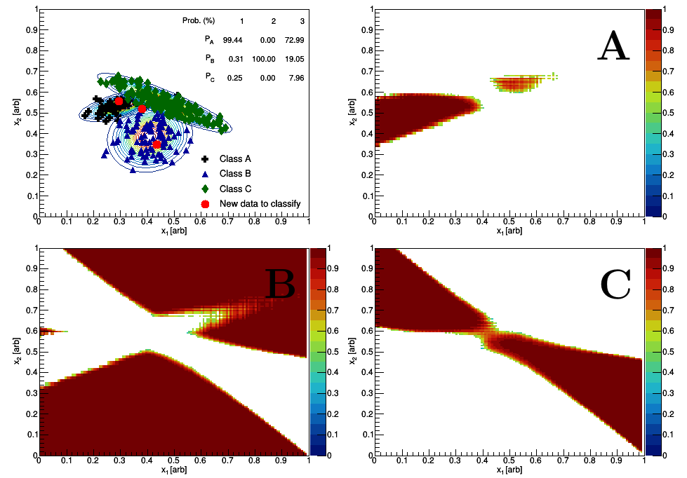
The training data, which may be seen by the blue triangles, black crosses, and green diamonds in Fig. 1, need to be analyzed in order to extract the mean $\boldsymbol{\mu} = ( \overline{x}_1, \overline{x}_2)^{\textrm{T}}$ and the covariance matrix $\boldsymbol{\Sigma}$ for each class. Assuming Gaussian class-conditionals, we may now calculate the 2-dimensional probability for the three classes, which may be seen by the contours in Fig. 1. The contours are built by scanning through the $x_1/x_2$ space and constructing a two-dimensional histogram where the color-weighting is the normalized multivariate Gaussian probability. We now have all the parts to make some predictions for unseen data.

Predictions

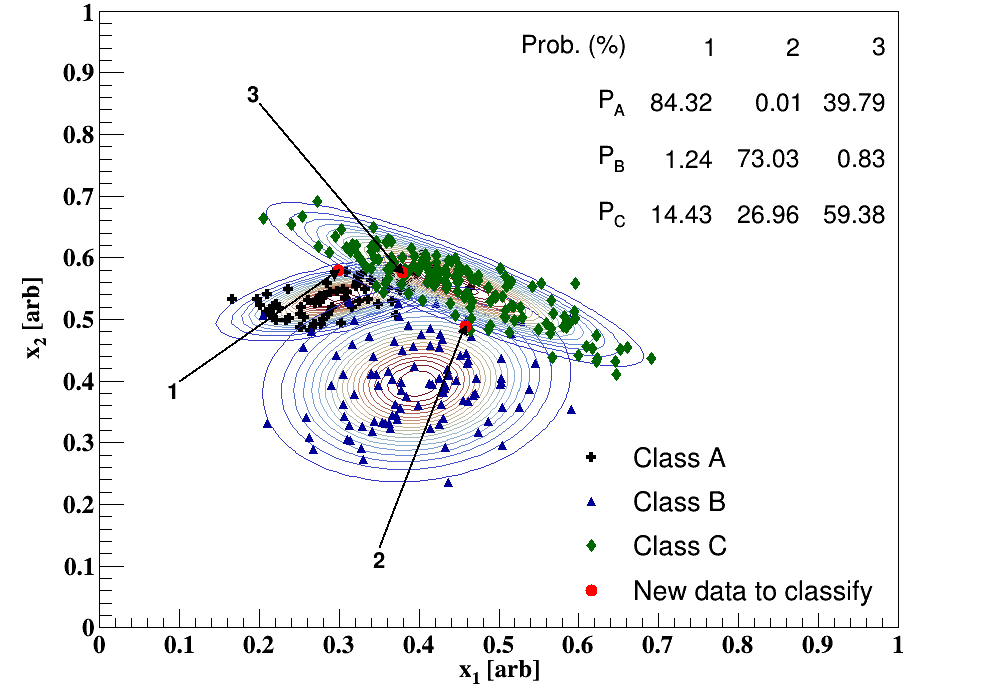
Fig. 1 has three unseen data labeled as 1-3. The points are randomly chosen using the Class probability distributions, i.e. point 1 is sampled from the Class A normal distribution; this is done on purpose as I know where the data came from and I want to see how the calculation classifies this object based on the above assumptions. In this case, the red circle labeled as 1 has an 84% chance of belonging to Class A, a 1% chance of belonging to Class B, and a 14% chance of belonging to Class C. This unseen point would therefore be classified as a member of Class A. Here is another example in which the calculations are explicitly shown, see the figure and table below.

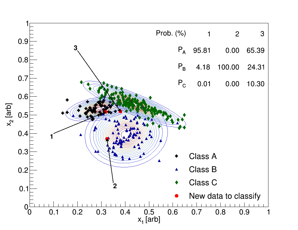
Point #	Class	Likelihood	Prior	Marginal	Posterior (%)
1	A	0.9754	0.2188	0.2227	95.813
1	B	0.0298	0.3125	0.2227	4.181
1	C	0.0000	0.4688	0.2227	0.006
2	A	0.0000	0.2188	0.0507	0.000
2	B	0.1621	0.3125	0.0507	100.000
2	C	0.0000	0.4688	0.0507	0.000
3	A	0.2168	0.2188	0.0724	65.394
3	B	0.0564	0.3125	0.0724	24.309
3	C	0.0159	0.4688	0.0724	10.297

Recall that the priors are calculated as the fraction of training objects in the class to the total number of training objects; therefore, since each class has a different number of points, the priors are different (Class A has 70, Class B has 100, and Class C has 150). The likelihood is calculated as the two-dimensional Gaussian using the mean and covariance matrix for that particular class, which is determined from the training data. The marginal is simply the sum of likelihood $\times$ prior for all three classes. The posterior, or the predictive probability of interest, is calculated as likelihood $\times$ prior/marginal. The point labeled as 3, which originally has been sampled from the Class C probability distribution, is determined to be a member of Class A, which is arguably incorrect.

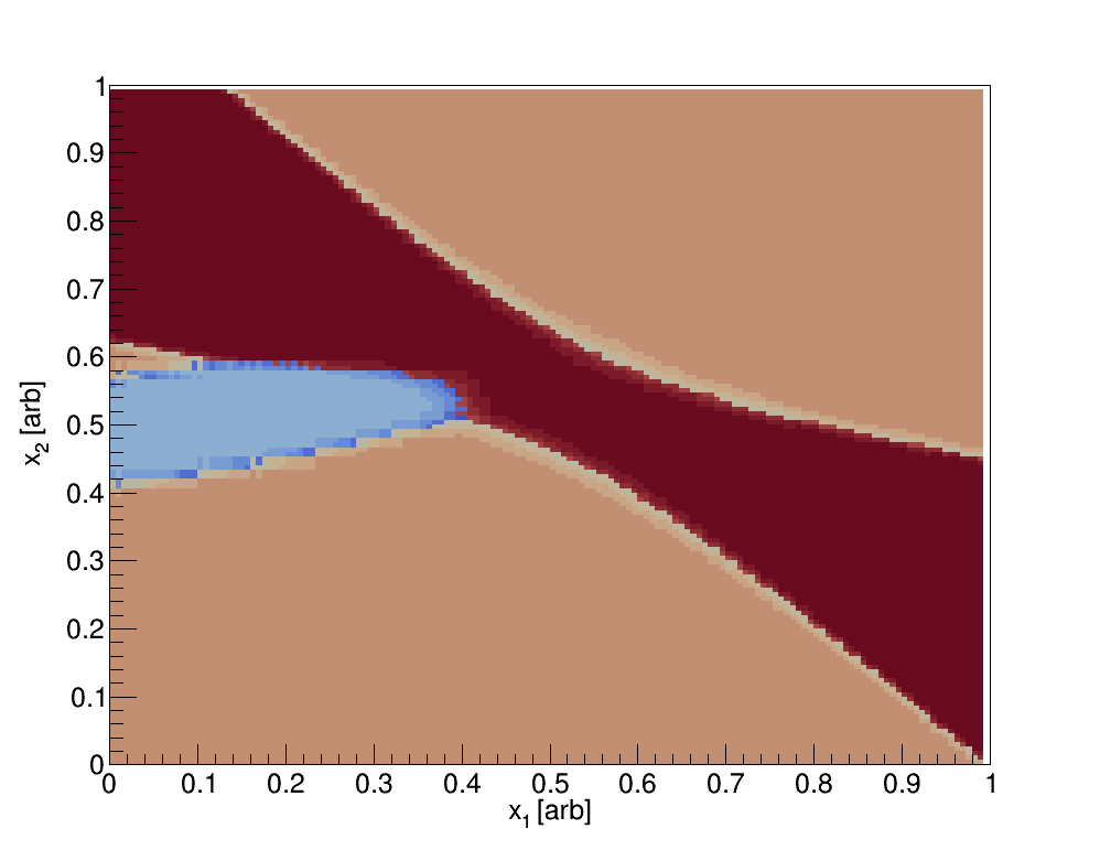
The classification may be summarized by the following histograms. One may scan through the feature space and calculate the posteriors for all classes; the maximum posterior then determines the classification, see the figure below where the light blue represents a situation where Class A is a maximum, tan represents when Class B is a maximum, and dark red represents when Class C is a maximum. Each class has a small gradient effect which is a result of the value of the class posterior when it’s determined to be the maximum. Lastly, see Fig. 3 for a summary of the three classes where in this case the color weighting is equal to the posterior probability.