Fractal Ferns

Barnsley Fern

The generation of ferns is surprisingly easy compared to other fractals that I’ve attempted; however, getting pretty color schemes was not obvious (at least for me). The fern idea is not mine, but a summary may be seen here. The technique falls under the category of an iterated function system which differs from the generation of a tree fractal or a Koch snowflake. In this case, very specific matrix transformations are performed on a point, and the type of transformation is dictated by a flat probability distribution. For example, the canonical fern is the so-called Barnsley fern, which may be generated by considering some initial point defined to be $x_n$. The initial point undergoes linear transformations of the type $x_{n+1} \rightarrow Mx_n + b$ where $M$ is a $2\times2$ linear transformation and $b$ is a translational term. The Barnsley fern is generated by the following choices of $M$ and $b$:

$\begin{align} \begin{pmatrix} x_{n+1} \\ y_{n+1} \end{pmatrix} &= \begin{pmatrix} 0.00 & 0.00 \\ 0.00 & 0.16 \end{pmatrix} \begin{pmatrix} x_n \\ y_n \end{pmatrix} + \begin{pmatrix} 0.00 \\ 0.00 \end{pmatrix} \hspace{1cm} P=0.01, \\ \begin{pmatrix} x_{n+1} \\ y_{n+1} \end{pmatrix} &= \begin{pmatrix} 0.85 & 0.04 \\ -0.04 & 0.85 \end{pmatrix} \begin{pmatrix} x_n \\ y_n \end{pmatrix} + \begin{pmatrix} 0.00 \\ 0.16 \end{pmatrix} \hspace{1cm} P=0.85, \\ \begin{pmatrix} x_{n+1} \\ y_{n+1} \end{pmatrix} &= \begin{pmatrix} 0.20 & -0.26 \\ 0.23 & 0.22 \end{pmatrix} \begin{pmatrix} x_n \\ y_n \end{pmatrix} + \begin{pmatrix} 0.00 \\ 1.60 \end{pmatrix} \hspace{1cm} P=0.07, \\ \begin{pmatrix} x_{n+1} \\ y_{n+1} \end{pmatrix} &= \begin{pmatrix} -0.15 & 0.28 \\ 0.26 & 0.24 \end{pmatrix} \begin{pmatrix} x_n \\ y_n \end{pmatrix} + \begin{pmatrix} 0.00 \\ 0.44 \end{pmatrix} \hspace{1cm} P=0.07. \\ \end{align}$

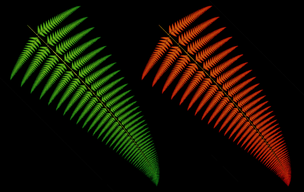
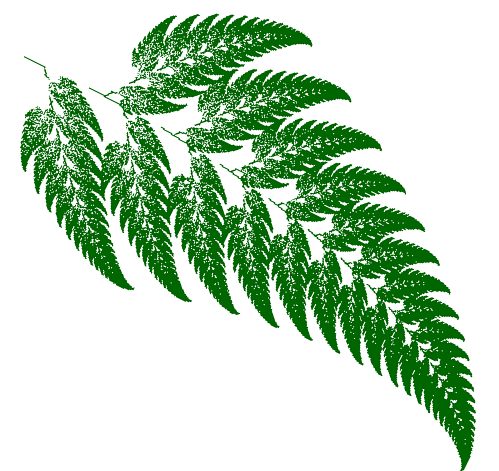
Which transformation to use depends on a flat random probability distribution denoted by $P$, so for example the first transformation is only applied 1% of the time while the second is applied 85%. The result is the famous Barnsley fern which may be seen by Fig. 2; the fern is generated by starting with some initial point and applying the formula with the defined probabilities many times, say $10^{5} - 10^{8}$. This is an $xy$ plot, though, not a histogram which is important when it comes to assigning colors to the fern. Note that this fern does not look exactly the same as Fig. 1 which are generated using the prescription found here:

$\begin{align} \begin{pmatrix} x_{n+1} \\ y_{n+1} \end{pmatrix} &= \begin{pmatrix} 0.00 & 0.00 \\ 0.00 & 0.20 \end{pmatrix} \begin{pmatrix} x_n \\ y_n \end{pmatrix} + \begin{pmatrix} 0.00 \\ -0.12 \end{pmatrix} \hspace{1cm} P=0.01, \\ \begin{pmatrix} x_{n+1} \\ y_{n+1} \end{pmatrix} &= \begin{pmatrix} 0.845 & 0.035 \\ -0.035 & 0.82 \end{pmatrix} \begin{pmatrix} x_n \\ y_n \end{pmatrix} + \begin{pmatrix} 0.00 \\ 1.60 \end{pmatrix} \hspace{1cm} P=0.85, \\ \begin{pmatrix} x_{n+1} \\ y_{n+1} \end{pmatrix} &= \begin{pmatrix} 0.20 & -0.31 \\ 0.255 & 0.245 \end{pmatrix} \begin{pmatrix} x_n \\ y_n \end{pmatrix} + \begin{pmatrix} 0.00 \\ 0.29 \end{pmatrix} \hspace{1cm} P=0.07, \\ \begin{pmatrix} x_{n+1} \\ y_{n+1} \end{pmatrix} &= \begin{pmatrix} -0.15 & 0.24 \\ 0.25 & 0.20 \end{pmatrix} \begin{pmatrix} x_n \\ y_n \end{pmatrix} + \begin{pmatrix} 0.00 \\ 0.68 \end{pmatrix} \hspace{1cm} P=0.07, \\ \end{align}$

which is quite similar to the Barnsley parameters with the exception of the translational terms. An animation of the fern development is seen by Fig. 4. The trick to getting the colors observed in Fig. 1 is to plot the fern in a two-dimensional histogram which contains more information than a simple xy plot. Why? Well, certain points are chosen more frequently than others, and this information may be captured by a histogram. For example, I used a large number of bins for the x and y variables, roughly 900 to 1000, and then the logarithm of the number events in each bin may be used to define the rgb value. The ferns in Fig. 1 are displayed in a log-scale which highlights small differences in bin counts; furthermore, the color gradient observed in the leaves (there is a proper name for this) occurs naturally.

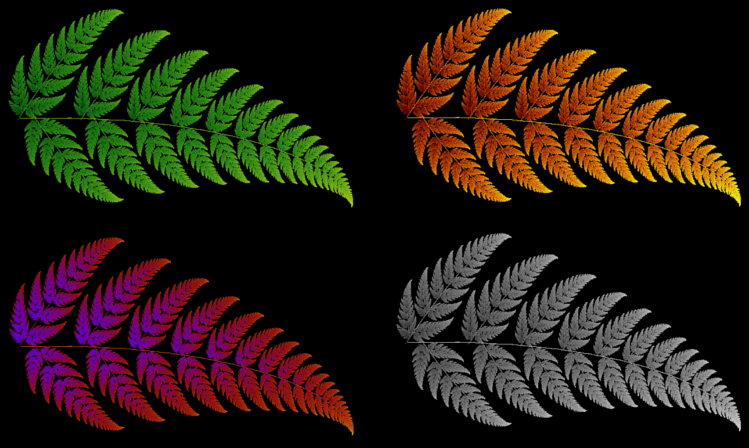
Another pretty fern may be generated using the following values for $M$ and $b$ (found on Wiki) and may be seen by Fig. 3:

$\begin{align} \begin{pmatrix} x_{n+1} \\ y_{n+1} \end{pmatrix} &= \begin{pmatrix} 0.00 & 0.00 \\ 0.00 & 0.25 \end{pmatrix} \begin{pmatrix} x_n \\ y_n \end{pmatrix} + \begin{pmatrix} 0.00 \\ -0.40 \end{pmatrix} \hspace{1cm} P=0.02, \\ \begin{pmatrix} x_{n+1} \\ y_{n+1} \end{pmatrix} &= \begin{pmatrix} 0.95 & 0.005 \\ -0.005 & 0.93 \end{pmatrix} \begin{pmatrix} x_n \\ y_n \end{pmatrix} + \begin{pmatrix} -0.002 \\ 0.50 \end{pmatrix} \hspace{1cm} P=0.84, \\ \begin{pmatrix} x_{n+1} \\ y_{n+1} \end{pmatrix} &= \begin{pmatrix} 0.035 & -0.20 \\ 0.16 & 0.04 \end{pmatrix} \begin{pmatrix} x_n \\ y_n \end{pmatrix} + \begin{pmatrix} -0.09 \\ 0.02 \end{pmatrix} \hspace{1cm} P=0.07, \\ \begin{pmatrix} x_{n+1} \\ y_{n+1} \end{pmatrix} &= \begin{pmatrix} -0.04 & 0.20 \\ 0.16 & 0.04 \end{pmatrix} \begin{pmatrix} x_n \\ y_n \end{pmatrix} + \begin{pmatrix} 0.083 \\ 0.12 \end{pmatrix} \hspace{1cm} P=0.07. \\ \end{align}$