Perceptron

The perceptron is a simple model for supervised learning of binary classifiers. The algorithm makes use of ROOT, which has vector and matrix classes for convenience. I generated two sets of pseudo-training data, which are normally distributed of varying means and sigmas, that are classified as blue circle = -1 and red triangle = +1, see Figure 1. One may think of a system that needs to classify a coin based on radius and mass for example. The classification function is $S = \boldsymbol{w} \cdot \boldsymbol{x} + b$, where $\boldsymbol{w}$ are the weights to be learned and are initially assigned random values, $\boldsymbol{x}$ are the features (mass and radius in this case), and $b$ is a threshold or bias constant. A common practice is to absorb $b$ into the zeroth component of $\boldsymbol{w}$ and to set the zeroth component of $\boldsymbol{x}$ to 1, which results in a vector $\boldsymbol{w}$ of size 3. Therefore, $\boldsymbol{w} \cdot \boldsymbol{x}$ is simply a vector dot-product. If $S>0$ ($S<0$) and the data point in question is a red triangle (blue circle), then the weight vector $\boldsymbol{w}$ has done a successful classification. On the other hand, if $S>0$ ($S<0$) and the data point in question is a blue circle (red triangle), then the weights (which determine the slope and intercept of the linear classification function) need to be updated. The update rule is: $\boldsymbol{w}(t+1) = \boldsymbol{w}(t) + \eta * h(t) * \boldsymbol{x}(t)$, where $\eta$ is a learning-rate constant chosen to be 0.05, $t$ is the iteration number, $h$ is the correct classification of the point in question (either +1 or -1), and $\boldsymbol{x}$ represents the features. In other words, incorrect classifications wiggle the linear decision boundary to a position where data are correctly classified, i.e. data of one type falls on one side of the line, and the remaining data falls on the other side.

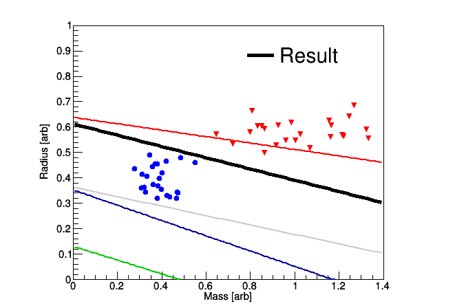
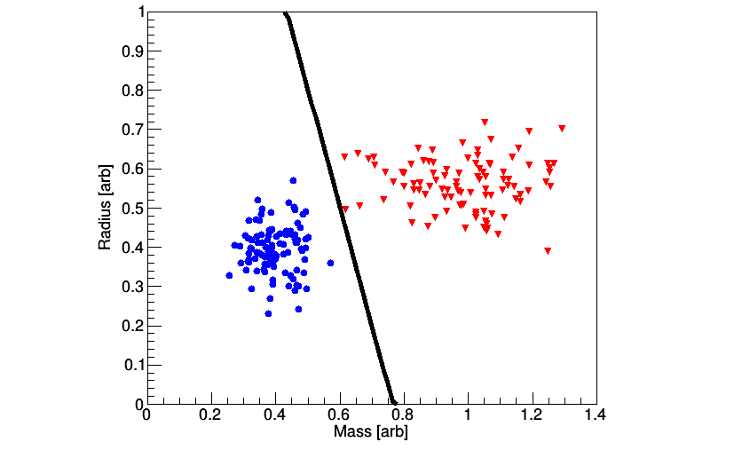
Assuming that the data is linearly separable, then the algorithm needs to examine the full data set many times. For each iteration, a for-loop through the full data set is implemented in which $S$ is calculated for each data point. If a data point is incorrectly classified, then update $\boldsymbol{w}$. If the for-loop scans through all data and no updates to $\boldsymbol{w}$ are performed, then successfully exit. A linear line may then be constructed with a slope of $-w_{1}/w_{2}$ and an intercept of $-w_{0}/w_{2}$, which are the components of the $\boldsymbol{w}$ vector. See Fig. 2 for an example of the updating, and note that the algorithm simply stops once a correct classification of the training data has been reached.

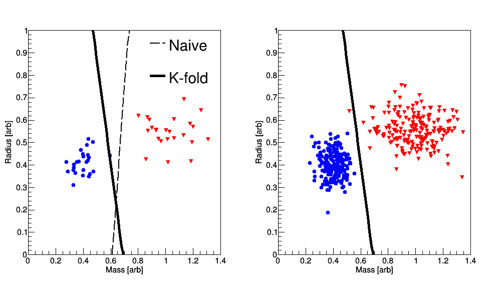
In order to improve upon the previous approach, the training data may be sub-divided many times in order to calculate $\boldsymbol{w}$ repeatedly for slightly different data sets and initial conditions. For this example, one data point is removed the from the training data set, and the algorithm is implemented using the $N-1$ data points; this procedure is repeated until every data point has been removed (while retaining the $N-1$ size, so put back the previously removed point), and the average $\boldsymbol{w}$ is taken as the final decision boundary. This approach is sometimes referred to as $K$-fold cross validation; see Fig. 3 where the left panel displays the training (bold line is the result of the $K$-fold averaging approach). The right panel shows how well the classifier does with unseen data, which in this case an efficiency of greater than 99% is observed.